Protoplanetary disk models

Protoplanetary disk models#

DiskSource provides parametric protoplanetary-disk sky models for lightweight interferometric workflows. Each component specifies a radial brightness profile, outer (and optionally inner) radius, inclination, and position angle. Visibilities are evaluated directly in the UV plane using closed-form Fourier transforms (or a small radial quadrature for power-law disks) — no hydrodynamics and no radiative transfer.

What this is for: fast sky simulation, imaging pipeline tests, AI/ML training data, and algorithm benchmarking. Compared to hydrodynamic or Monte Carlo radiative-transfer models, these analytic disks are lighter, easier to configure, and much faster to evaluate (especially at scale with Dask). You trade physical realism for speed and reproducibility when the goal is to test interferometry software, not to model gas dynamics.

What this is not: a substitute for realistic disk physics (gaps from planet formation, chemistry, time evolution, etc.). Use parametric rings and envelopes to mimic observed morphology, then validate imaging or ML methods against known ground truth in the visibility domain. Compose multiple components with CompositeSource (or the + operator) — see examples/notebooks/protoplanetary_disk_alma_simulation.ipynb.

Geometry: inclination and position angle#

Disk radii are defined in the disk midplane. Inclination \(i\) and position angle \(\mathrm{PA}\) project the disk onto the sky and rotate the UV coordinates used by the Fourier transform. The formulas below follow projected_uv_radius().

Position angle convention: \(\mathrm{PA}\) is the major-axis orientation east of north — the same definition as FITS BPA, CASA restoring beams, and radio_beam.Beam (counterclockwise from north on the sky). This matches ALMA protoplanetary-disk papers. Internally the rotation uses \(\theta = \pi/2 - \mathrm{PA}\) because \(l\) is defined positive toward east and \(m\) toward north.

Sky direction-cosine offsets \((l, m)\) are in radians (small-angle limit: \(\Delta\mathrm{RA} \approx l / \cos\delta\)). \(l\) is positive toward east; \(m\) is positive toward north. Pyralysis builds image-plane coordinates like create_image_meshgrid():

\[l = (i - i_0)\,\mathrm{cellsize}_l,\quad m = (j - j_0)\,\mathrm{cellsize}_m\]

with \(\mathrm{cellsize}_l = \texttt{cellsize[0]} < 0\) and \(\mathrm{cellsize}_m = \texttt{cellsize[1]} > 0\). The negative horizontal cellsize is what makes \(\Delta\mathrm{RA}\) run left to right from positive to negative on displayed images. With \(\theta = \pi/2 - \mathrm{PA}\), after rotation into the disk frame,

\[l_r = l\cos\theta + m\sin\theta,\quad m_r = -l\sin\theta + m\cos\theta\]

\[\rho = \sqrt{l_r^2 + \left(\frac{m_r}{\cos i}\right)^2}\]

where \(l_r\) lies along the projected major axis and \(m_r\) along the minor axis. The same \(\rho\) projection enters the UV-plane visibility factor via projected_uv_radius().

In the UV plane, coordinates \((u, v)\) in wavelengths use the same \(\theta\) and \(\cos i\) projection as in the class docstring of DiskSource.

GaussianSource uses the same \(\mathrm{PA}\) convention for theta_angle.

Note

Bright ring lobes in inclined disks trace the minor axis (limb brightening), not the geometric major axis. When comparing dirty images to model \(\mathrm{PA}\), measure the envelope orientation or use visibility-domain geometry checks rather than peak-to-peak separation alone.

Model images (sky brightness)#

Before convolution with the instrumental response, the disk appears on the sky as a 2D brightness distribution \(I(l, m)\). The figures below are normalized model images (not dirty maps or simulated visibilities) rasterized with the Pyralysis cellsize sign convention above.

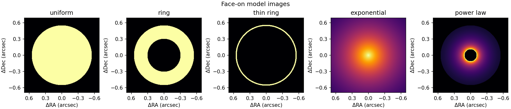
Face-on normalized model images for the five built-in profiles (\(i = 0^\circ\)). \(\Delta\mathrm{RA}\) increases to the left.#

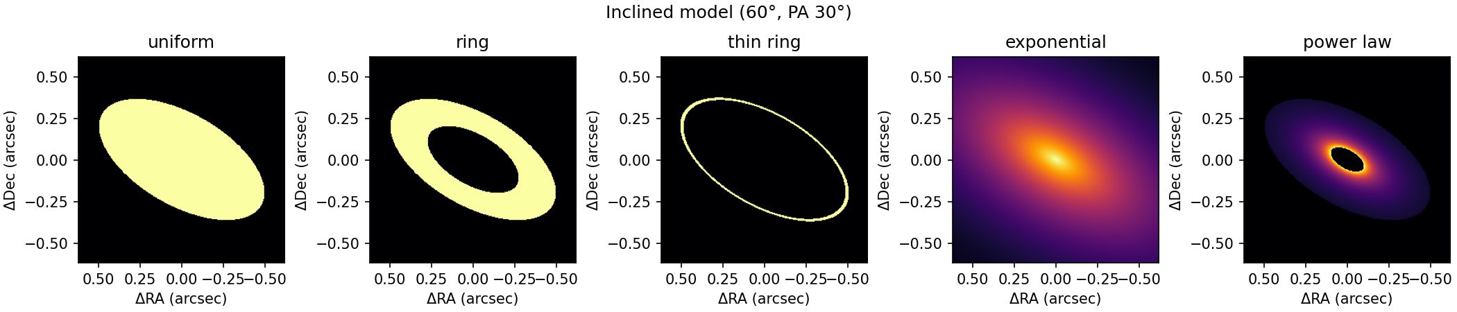
Same profiles at \(i = 60^\circ\), \(\mathrm{PA} = 30^\circ\). The projected ellipse flattens by \(\cos i\) along the minor axis.#

Sky brightness shapes (normalized to peak 1):

Profile	\(I(\rho)\) in the disk midplane (\(\rho\) in rad)
`uniform`	Constant inside \(\rho \le r_\mathrm{out}\); zero outside
`ring`	Constant for \(r_\mathrm{in} \le \rho \le r_\mathrm{out}\)
`thin_ring`	Infinitely thin shell at \(\rho = r_\mathrm{out}\); the documentation figure uses a narrow annulus for display only
`exponential`	\(\exp(-\rho / r_\mathrm{out})\)
`power_law`	\(\rho^{-p}\) between \(r_\mathrm{in}\) and \(r_\mathrm{out}\) (peak-normalized for display)

Regenerate the documentation figures after changing profile math (one-off script, not part of the installed package):

python docs/scripts/generate_disk_profile_figures.py

UV-plane visibilities (Fourier theory)#

DiskSource returns visibilities

\[V(u,v) = I_0 \times F(u,v) \times e^{-2\pi i (u l_0 + v m_0 + w (n_0 - 1))}\]

where \(I_0\) is the Stokes flux from reference_intensity, \(F\) is the normalized spatial Fourier factor from disk_profile_visibility(), and the phase term shifts the disk when sky_position is offset from the phase center.

With \(x = 2\pi r_\mathrm{out}\,\rho\) and \(\rho\) the projected UV radius above, the analytic factors implemented in pyralysis.models.sky.disk_profiles are:

Uniform disk

\[F_\mathrm{uniform}(\rho) = \frac{2 J_1(x)}{x}\]

Annular ring (\(r_\mathrm{in} < r_\mathrm{out}\))

\[F_\mathrm{ring}(\rho) = \frac{r_\mathrm{out}^2}{r_\mathrm{out}^2 - r_\mathrm{in}^2} \frac{2 J_1(2\pi r_\mathrm{out}\rho)}{2\pi r_\mathrm{out}\rho} - \frac{r_\mathrm{in}^2}{r_\mathrm{out}^2 - r_\mathrm{in}^2} \frac{2 J_1(2\pi r_\mathrm{in}\rho)}{2\pi r_\mathrm{in}\rho}\]

Thin ring at \(r_\mathrm{out}\)

\[F_\mathrm{thin}(\rho) = J_0(2\pi r_\mathrm{out}\rho)\]

Exponential disk

\[F_\mathrm{exp}(\rho) = \left(1 + x^2\right)^{-3/2}\]

Note

The disk exponential profile is not GaussianSource. A Gaussian has image brightness \(\propto \exp(-r^2/2\sigma^2)\) and UV visibility \(\exp(-2\pi^2\sigma^2\rho^2)\); the disk exponential has \(\exp(-\rho/r_\mathrm{out})\) in the midplane and \(F_\mathrm{exp}=(1+x^2)^{-3/2}\) above. Use GaussianSource for elliptical Gaussians; use profile_type="exponential" for a radial disk envelope.

Power law \(\rho^{-p}\) between \(r_\mathrm{in}\) and \(r_\mathrm{out}\)

\[F_\mathrm{pl}(\rho) = \int_{r_\mathrm{in}}^{r_\mathrm{out}} r^{1-p}\, J_0(2\pi r \rho)\, dr \Big/ \int_{r_\mathrm{in}}^{r_\mathrm{out}} r^{1-p}\, dr\]

The implementation uses a fixed 100-point radial quadrature (see _POWER_LAW_QUADRATURE_STEPS in pyralysis.models.sky.disk_profiles).

All factors are evaluated in float32 with Dask block-wise SciPy Bessel calls for HPC-friendly simulation.

Building individual disk components#

Angle attributes accept Quantity, Angle, strings, or numeric literals (radii in radians, orientation angles in degrees when passed as bare numbers), matching GaussianSource.

Uniform disk

from astropy import units as u
from pyralysis.models.sky import DiskSource

inner_disk = DiskSource(
    reference_intensity=0.5 * u.Jy,
    reference_frequency=230e9 * u.Hz,
    sky_position="16h00m00s -30d00m00s",
    profile_type="uniform",
    major_radius=0.12 * u.arcsec,
    inclination=45 * u.deg,
    position_angle=30 * u.deg,
)

Bright ring

bright_ring = DiskSource(
    reference_intensity=2.5 * u.Jy,
    reference_frequency=230e9 * u.Hz,
    sky_position="16h00m00s -30d00m00s",
    profile_type="ring",
    inner_radius=0.35 * u.arcsec,
    major_radius=0.55 * u.arcsec,
    inclination=45 * u.deg,
    position_angle=30 * u.deg,
)

Thin ring (delta shell in the UV plane)

thin_ring = DiskSource(
    reference_intensity=1.0 * u.Jy,
    profile_type="thin_ring",
    major_radius=0.5 * u.arcsec,
    inclination=60 * u.deg,
    position_angle=30 * u.deg,
)

Exponential envelope

envelope = DiskSource(
    reference_intensity=1.0 * u.Jy,
    profile_type="exponential",
    major_radius=0.7 * u.arcsec,
    inclination=45 * u.deg,
    position_angle=30 * u.deg,
)

Power-law disk

power_disk = DiskSource(
    reference_intensity=1.0 * u.Jy,
    profile_type="power_law",
    inner_radius=0.2 * u.arcsec,
    major_radius=1.0 * u.arcsec,
    power_index=1.5,
    inclination=45 * u.deg,
    position_angle=30 * u.deg,
)

Composing multi-component disks#

Add components with CompositeSource or +. Negative reference_intensity on a ring can carve a parametric gap without a dedicated gap profile.

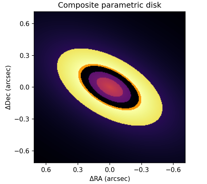
Composite parametric disk model image — Example composite: exponential envelope + bright ring − darker ring + compact uniform core (same geometry as the ALMA notebook).#

from pyralysis.models.sky import CompositeSource, DiskSource

common = dict(
    sky_position="16h00m00s -30d00m00s",
    reference_frequency=230e9,
    inclination=45,
    position_angle=30,
)

disk_model = CompositeSource(
    sources=[
        DiskSource(
            reference_intensity=1.0,
            profile_type="exponential",
            major_radius="0.7 arcsec",
            **common,
        ),
        DiskSource(
            reference_intensity=2.5,
            profile_type="ring",
            inner_radius="0.35 arcsec",
            major_radius="0.55 arcsec",
            **common,
        ),
        DiskSource(
            reference_intensity=-0.8,
            profile_type="ring",
            inner_radius="0.22 arcsec",
            major_radius="0.32 arcsec",
            **common,
        ),
        DiskSource(
            reference_intensity=0.5,
            profile_type="uniform",
            major_radius="0.12 arcsec",
            **common,
        ),
    ],
    operation="add",
)

Simulating visibilities#

Once the sky model is defined, pass it to Simulator as for any other source. Pyralysis evaluates visibilities analytically in the UV plane. The model-image figures earlier show true sky brightness; a dirty map is that brightness convolved with the synthesised beam and affected by UV-coverage sidelobes.

The ALMA notebook (protoplanetary_disk_alma_simulation.ipynb) uses the same composite disk_model geometry as above. Its observation setup is:

Array: alma.cycle9.7.cfg (43 antennas, long-baseline Cycle 9)
Band 6: 10 channels of 100 MHz from 229.55 to 230.45 GHz (centred on 230 GHz)
Time: 10 minutes total, 2-minute integrations (five time steps)
Imaging: cellsize = \mathrm{theo\_resolution}/7, fixed imsize = 2048 (use 1024 for a faster run), Natural weighting, then DirtyMapper
Display: crop ±1 arcsec around the phase centre so rings are easy to see

Omit explicit chunks on Simulator so Dask uses "auto". Expect similar morphology between model images and the dirty map, not a pixel-identical match.

Tip

Resolved structure needs radii comparable to or larger than the synthesized beam. With ALMA Band 6 and long-baseline configurations the beam can be \(\sim 0.07''\) or finer; use arcsecond-scale radii in tutorials unless you deliberately want an unresolved component.

from astropy import units as u
from astropy.coordinates import Angle
from astropy.time import Time

from pyralysis.io.antenna_config_io import AntennaConfigurationIo
from pyralysis.simulation import Simulator

interferometer = AntennaConfigurationIo(
    input_name="src/pyralysis/simulation/antenna_configs/alma.cycle9.7.cfg"
).read()
interferometer.configure_observation(
    min_frequency=229.55e9,
    max_frequency=230.55e9,  # half-open grid → 10 × 100 MHz channels to 230.45 GHz
    frequency_step=100e6,
    right_ascension=Angle("16h00m00s", unit=u.hourangle),
    declination=Angle("-30d00m00s"),
    integration_time=2 * u.minute,
    observation_time="10m",
    reference_time=Time("2024-01-01T00:00:00", format="isot"),
)

dataset = Simulator(interferometer=interferometer, sources=disk_model).simulate(
    create_dataset=True
)

The notebook continues with ThermalNoiseInjector (channel_bandwidth=100 MHz, integration_time=2 min), Natural weighting, and dirty imaging. See Simulation Framework for noise injection, chunking, and dataset export.

Protoplanetary disk models

Contents