Objective Function Framework

Objective Function Framework#

Overview#

Pyralysis provides a sophisticated optimization framework built around flexible, composable objective functions. The system is designed for both research and production use, with support for modern optimization algorithms and scalable processing.

Note

The optimization framework uses a term-based architecture where each component is implemented as a separate class, providing modularity, flexibility, and extensibility.

Architecture#

The optimization framework consists of several key components:

ObjectiveFunction: Main container that combines multiple terms
ObjectiveFunctionTerm: Base class for all terms (data fidelity, regularization)
Data Fidelity Terms: ChiSquared, AmplitudeChiSquared, PhaseChiSquared
Regularization Terms: L1Norm, Entropy, Tikhonov, TotalFlux, TSV

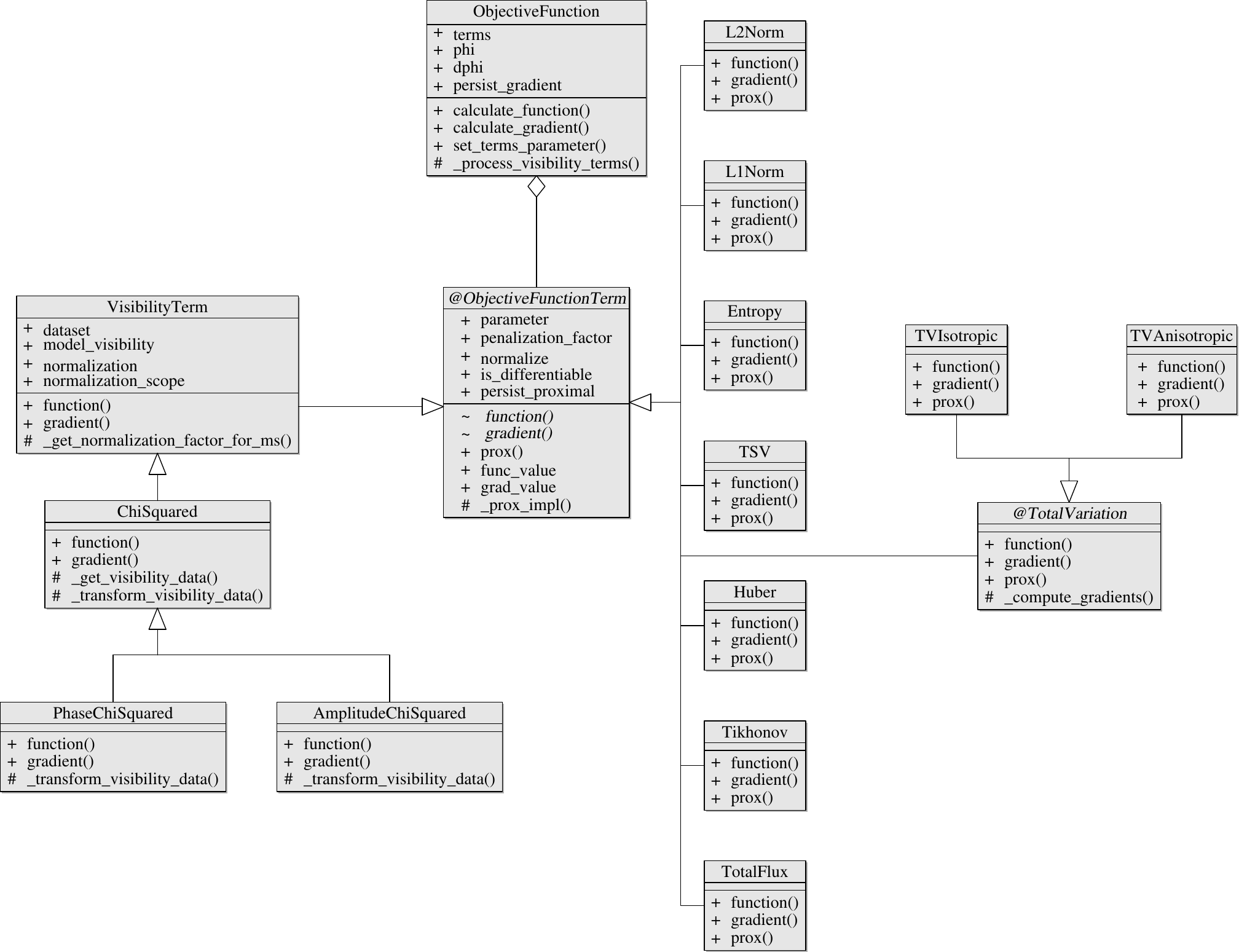
Objective function and term hierarchies — **Objective function architecture** (`ObjectiveFunction` and objective terms).#

Key Benefits#

Modularity: Add, remove, or modify terms without changing the core framework
Flexibility: Combine any number of terms with different weights
Extensibility: Easy to implement new regularization or data fidelity terms
Performance: Efficient computation with optional gradient caching

Data Fidelity Terms#

Pyralysis provides several chi-squared data fidelity terms for different types of visibility data fitting:

Chi-Squared (Standard)#

Standard complex visibility chi-squared for full Stokes data. The Stokes planes fitted are those present on the parameter Image (from CLI --stokes or pipeline config); correlation↔Stokes conversion follows those labels.

Mathematical Formulation:

\[\chi^2 = \frac{1}{2} \sum_k w_k \|V_k^o - V_k^m(I)\|^2\]

Typical Use Case: Standard interferometric imaging with complex visibilities.

Implementation:

from pyralysis.optimization.terms import ChiSquared

chi2_term = ChiSquared(
    model_visibility=mv,
    normalization="effective_samples",  # Default normalization mode
    normalization_scope="whole_dataset",  # Default scope
    penalization_factor=1.0
)

Amplitude Chi-Squared#

Amplitude-only chi-squared using individual visibility amplitudes.

Mathematical Formulation:

\[\chi^2_A = \frac{1}{2} \sum_k \left(\frac{\|V_k^o\| - \|V_k^m(I)\|}{\sigma_k}\right)^2\]

Typical Use Case: Amplitude-only imaging, when phase calibration is unreliable.

Implementation:

from pyralysis.optimization.terms import AmplitudeChiSquared

amp_term = AmplitudeChiSquared(
    model_visibility=mv,
    penalization_factor=1.0
)

Phase Chi-Squared#

Phase-only chi-squared using unit phasors of individual visibilities.

Mathematical Formulation:

\[\chi^2_P = \frac{1}{2} \sum_k w_k \left\|\frac{V_k^o}{\|V_k^o\|} - \frac{V_k^m}{\|V_k^m\|}\right\|^2\]

Typical Use Case: Phase-only imaging, robust to amplitude calibration errors.

Implementation:

from pyralysis.optimization.terms import PhaseChiSquared

phase_term = PhaseChiSquared(
    model_visibility=mv,
    penalization_factor=1.0
)

Normalization Modes#

Visibility terms support flexible normalization strategies that scale objective function (OF) values and gradients. The numerical magnitude of χ² therefore depends on the chosen mode. Use normalization when you want a more stable scale across datasets of different size or weight structure; do not treat OF values from different modes as interchangeable.

Visibility-term default (API and optimization CLI): normalization="effective_samples" with scope WHOLE_DATASET. Selecting another mode requires an explicit normalization=... argument.
Values are not comparable across modes. Changing none ↔ sum_weights ↔ effective_samples changes the OF / χ² scale; do not compare λ schedules or convergence histories across different normalizers without re-tuning.
Normalized χ² is not automatically “reduced χ² ≈ 1”. Only some weight+noise setups make effective_samples (or another mode) behave like a classical reduced χ². See Visibility data weights for matching thermal noise and imaging weights.
Two different knobs exist:
- Visibility terms: normalization= (string / strategy; default effective_samples).
- Regularizers (and the inherited base flag): normalize: bool = False — pixel-count / DOF scaling for image-domain terms. This flag is orthogonal to visibility normalization= today: passing normalize=True to ChiSquared does not switch the visibility strategy to visibility_number.

Available Normalization Modes:

Normalization Modes#
Mode	Description	Use Case
`"none"`	No normalization (factor = 1.0)	When absolute chi-squared values are needed
`"visibility_number"`	Normalize by number of unflagged visibilities	Comparing datasets with different visibility counts
`"sum_weights"`	Normalize by sum of imaging weights	Accounting for total data weight rather than count
`"effective_samples"`	Normalize by effective number of samples from weights	When weights are non-uniform (default for ChiSquared)

Normalization Scopes:

PER_SUBMS: Each measurement set (SubMS) gets its own normalization factor
WHOLE_DATASET: Single normalization factor computed across all measurement sets (default for ChiSquared)

Default Behavior:

ChiSquared (and other visibility terms) use effective_samples with WHOLE_DATASET by default. That accounts for weight variance and is usually a good default scale, but it does not by itself guarantee reduced-χ² ≈ 1. For simulated datasets, keep IMAGING_WEIGHT_SPECTRUM aligned with the injected noise level; Visibility data weights explains how thermal-noise injection and the analytic/empirical estimators populate those weights.

Mathematical Formulations:

Visibility Number Normalization:

\[\chi^2_{norm} = \frac{\chi^2}{N}\]

where \(N\) is the number of unflagged visibilities.

Sum of Weights Normalization:

\[\chi^2_{norm} = \frac{\chi^2}{\sum_k w_k}\]

where \(w_k\) are the imaging weights.

Effective Samples Normalization:

\[ \begin{align}\begin{aligned}N_{eff} = \frac{(\sum_k w_k)^2}{\sum_k w_k^2}\\\chi^2_{norm} = \frac{\chi^2}{N_{eff}}\end{aligned}\end{align} \]

This accounts for the variance in weights and provides a more accurate measure of effective sample size when weights are not uniform.

Usage Examples:

from pyralysis.optimization.terms import ChiSquared
from pyralysis.optimization.terms.normalization import NormalizationScope

# Default: effective_samples + WHOLE_DATASET
chi2_default = ChiSquared(model_visibility=mv)

# Custom normalization: sum of weights per SubMS
chi2_per_subms = ChiSquared(
    model_visibility=mv,
    normalization="sum_weights",
    normalization_scope=NormalizationScope.PER_SUBMS
)

# Visibility number normalization for whole dataset
chi2_vis_num = ChiSquared(
    model_visibility=mv,
    normalization="visibility_number",
    normalization_scope=NormalizationScope.WHOLE_DATASET
)

# No normalization
chi2_no_norm = ChiSquared(
    model_visibility=mv,
    normalization="none"
)

# Regularizer pixel DOF (separate from visibility normalization=)
from pyralysis.optimization.terms import L1Norm
l1 = L1Norm(penalization_factor=1e-3, normalize=True)

Performance Optimization:

Normalization factors are computed using cached lazy dask arrays, allowing dask to optimize the computation graph. Weight sums are cached at both SubMS and Dataset levels, with automatic cache invalidation when weights change.

When to Use Each Mode:

effective_samples (default): Best for most cases, especially when weights vary significantly
sum_weights: Use when you want to account for total data weight
visibility_number: Use for simple count-based normalization
none: Use when absolute chi-squared values are required

When to Use Each Scope:

WHOLE_DATASET: Use when comparing different datasets or when you want a single normalization factor
PER_SUBMS: Use when each measurement set should be normalized independently

Building Complex Objective Functions#

Create sophisticated objective functions by combining multiple terms:

from pyralysis.optimization import ObjectiveFunction
from pyralysis.optimization.terms import Chi2, L1Norm, TSV, Entropy

# Create a sophisticated objective function
terms = [
    # Data fidelity: fit observed visibilities
    Chi2(model_visibility=mv),  # default normalization=effective_samples

    # Regularization: promote sparsity
    L1Norm(penalization_factor=0.01),

    # Regularization: edge-preserving smoothness
    TSV(penalization_factor=0.005),

    # Regularization: bias toward prior image
    Entropy(prior_image=prior_model, penalization_factor=0.001)
]

# Initialize with performance optimizations
obj_func = ObjectiveFunction(
    terms=terms,
    parameter=image,
    persist_gradient=True,  # Cache gradients for performance
    chunks="auto"           # Automatic Dask chunking
)

Performance Features#

Gradient Persistence: Optional caching to avoid recomputation
Proximal Persistence: Optional caching of proximal operator results for FISTA/SDMM
Smart Term Processing: Efficient handling of shared computations
Dask Integration: Scalable parallel processing for large datasets
Memory Management: Configurable chunking and memory usage
Multi-channel Support: Handle spectral and polarization data efficiently

Gradient Persistence#

Enable gradient caching for improved performance:

obj_func = ObjectiveFunction(
    terms=terms,
    parameter=image,
    persist_gradient=True  # Cache gradients for performance
)

# Gradients are cached after first computation
obj_func.calculate_gradient(iteration=1)
obj_func.calculate_gradient(iteration=2)  # Uses cached gradients

Proximal Operator Persistence#

For proximal optimization methods (FISTA, SDMM), enable persistence of proximal operator results to maintain consistent iteration times:

from pyralysis.optimization.terms.regularizers import L1Norm, Tikhonov

# Enable proximal persistence for regularizers
l1_term = L1Norm(penalization_factor=0.01, persist_proximal=True)
tikh_term = Tikhonov(penalization_factor=0.001, persist_proximal=True)

# Proximal results are persisted in memory after computation
# This maintains consistent iteration times in FISTA/SDMM
# Similar to persist_gradient for differentiable terms

Chunking Configuration#

Configure Dask chunking for optimal performance:

# Manual chunking
obj_func = ObjectiveFunction(
    terms=terms,
    parameter=image,
    chunks=(256, 256)  # 256x256 pixel chunks
)

# Automatic chunking
obj_func = ObjectiveFunction(
    terms=terms,
    parameter=image,
    chunks="auto"  # Let Dask choose optimal chunks
)

Multi-channel Support#

Handle multi-channel images efficiently:

# Single channel optimization
single_channel = ObjectiveFunction(
    terms=[Chi2(mv), L1Norm(0.01)],
    parameter=image[:, :, 0],  # Single channel
    chunks="auto"
)

# Multi-channel optimization
multi_channel = ObjectiveFunction(
    terms=[Chi2(mv), L1Norm(0.01)],
    parameter=image,  # All channels
    chunks="auto"
)

Using the Objective Function#

Evaluate function values and gradients:

# Evaluate objective function
function_value = obj_func.calculate_function()
print(f"Objective function value: {function_value}")

# Calculate gradient
obj_func.calculate_gradient(iteration=1)

# Access gradient
gradient = obj_func.dphi

# Use in optimization loop
for iteration in range(max_iterations):
    function_value = obj_func.calculate_function()
    obj_func.calculate_gradient(iteration=iteration)
    # ... optimization step ...

Advanced Features#

Term Management: Add, remove, or modify terms dynamically
Parameter Updates: Update parameters without recreating the objective function
Masking: Apply operations only to specific regions
Normalization: Optional normalization of function values and gradients
Iteration Tracking: Built-in iteration counting for optimization algorithms

Term Management#

Modify objective function terms dynamically:

# Add new term
obj_func.terms.append(TSV(penalization_factor=0.01))

# Remove term
obj_func.terms.pop()  # Remove last term

# Modify existing term
obj_func.terms[1].penalization_factor = 0.02

Parameter Updates#

Update parameters efficiently:

# Update parameter for all terms
obj_func.terms_parameter(new_image)

# Update dataset for relevant terms
obj_func.terms_dataset(new_dataset)

# Update penalization factors
obj_func.terms_penalization([0.01, 0.005, 0.001])

Best Practices#

Start Simple: Begin with basic terms and add complexity gradually
Balance Terms: Ensure data fidelity and regularization are properly balanced
Use Persistence: Enable gradient persistence for repeated evaluations
Configure Chunking: Use appropriate chunking for your data size
Monitor Performance: Watch memory usage and computation time
Validate Results: Always check that the objective function behaves as expected

Example: Progressive Complexity

# Start with basic objective function
basic_terms = [Chi2(mv)]  # default normalization=effective_samples
basic_obj = ObjectiveFunction(terms=basic_terms, parameter=image)

# Add regularization gradually
basic_terms.append(L1Norm(0.01))
basic_obj.terms = basic_terms

# Add more sophisticated regularization
basic_terms.append(TSV(0.005))
basic_obj.terms = basic_terms

Regularization Methods | Optimization in Pyralysis | Optimizers | Line Searchers

Objective Function Framework

Contents

Objective Function Framework#

Overview#

Architecture#

Key Benefits#

Data Fidelity Terms#

Chi-Squared (Standard)#

Amplitude Chi-Squared#

Phase Chi-Squared#

Normalization Modes#

Building Complex Objective Functions#

Performance Features#

Gradient Persistence#

Proximal Operator Persistence#

Chunking Configuration#

Multi-channel Support#

Using the Objective Function#

Advanced Features#

Term Management#

Parameter Updates#

Best Practices#