Gridding Techniques in Pyralysis

Gridding Techniques in Pyralysis#

Why gridding matters#

Gridding is a fundamental step in radio interferometric imaging. It allows you to transform irregularly sampled visibility data into a form suitable for fast image reconstruction.

Pyralysis provides two main gridding approaches:

1️⃣ Count-in-Cell Gridding

A simple binning method that places visibilities into the nearest grid cell.
Fast, but introduces aliasing artifacts due to the sharp edges in Fourier space.

Note

For most applications, we recommend convolutional gridding for best results.

2️⃣ Convolutional Gridding (Recommended)

Uses a convolution kernel to interpolate visibilities onto the Fourier grid.
Reduces aliasing artifacts and improves reconstruction quality.

—

Basic Gridding with Gridder#

You can construct Gridder in two equivalent ways: pass grid= with an existing Grid, or pass imsize, cellsize, padding_factor, hermitian_symmetry, and optionally image so a Grid is built inside __post_init__. If grid is set, the other grid-related arguments are ignored for construction. Use gridder.grid to share the same instance with weighting schemes and other components.

DirtyMapper and MeasurementOperator subclass Gridder and forward keyword arguments to Gridder.__init__, so the same grid= and imsize / cellsize / padding_factor / hermitian_symmetry (and image) options apply there as well.

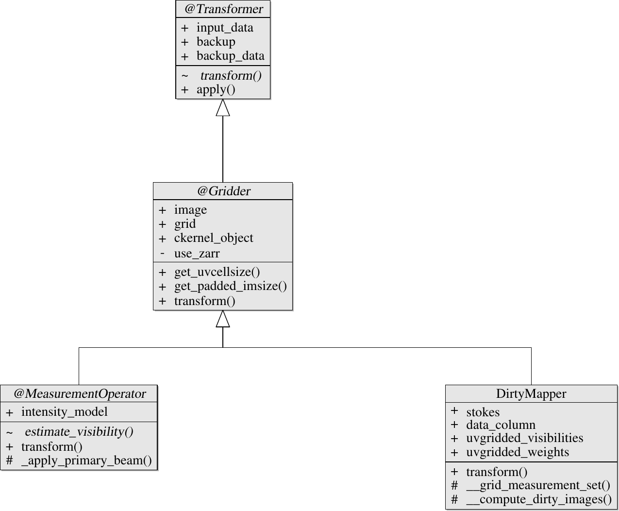
Transformer hierarchy including Gridder and MeasurementOperator — **Transformer hierarchy (page 1)** with `Gridder`, `MeasurementOperator` and `DirtyMapper`.#

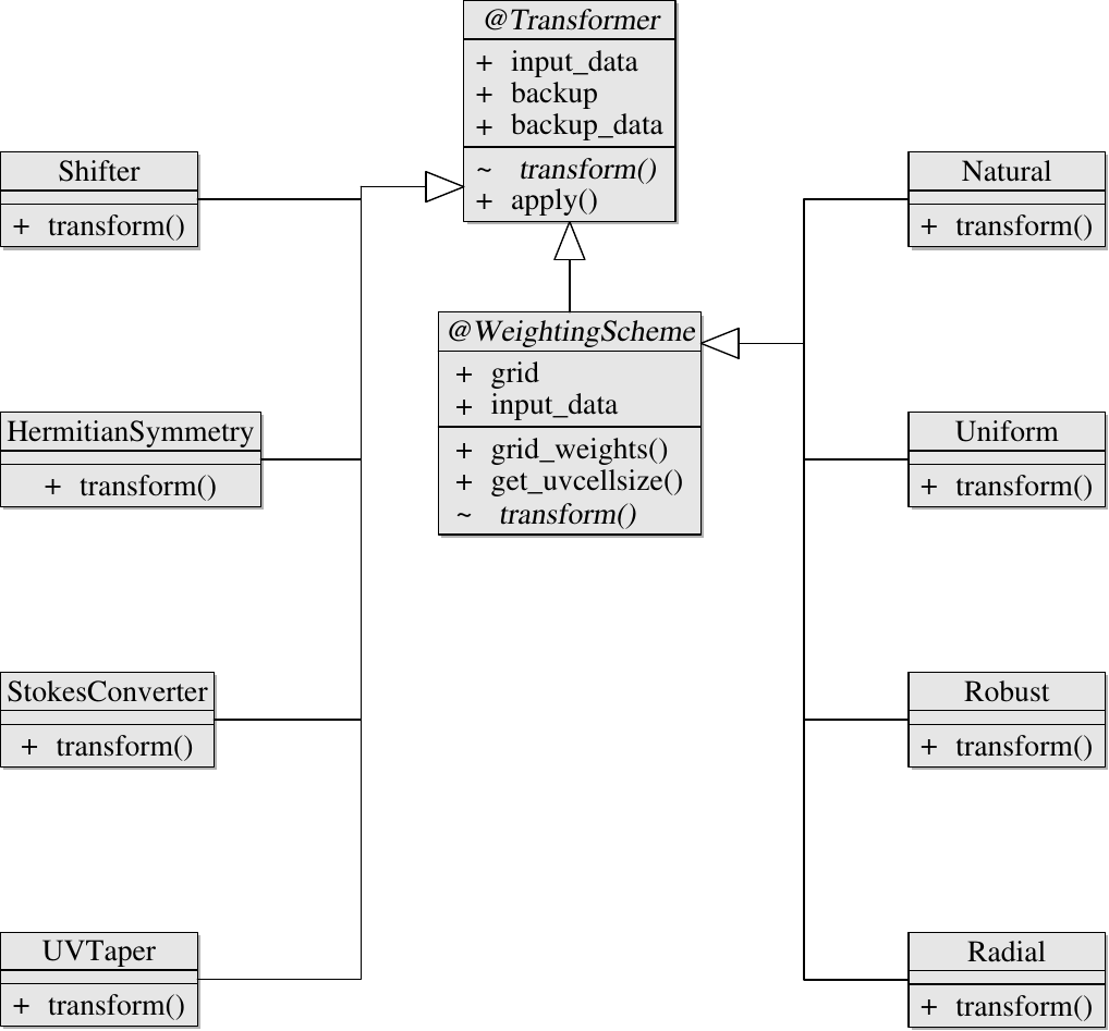
Transformer utilities and weighting schemes — **Transformer hierarchy (page 2)** with utilities and weighting schemes.#

From parameters (Grid is built inside Gridder):

import astropy.units as u
from pyralysis.transformers import Gridder

gridder = Gridder(
    imsize=512,
    cellsize=0.003 * u.arcsec,
    hermitian_symmetry=False,
    padding_factor=1.2
)
print(gridder.grid.imsize)  # [512, 512]

From an existing Grid:

import astropy.units as u
from pyralysis.grids import Grid
from pyralysis.transformers import Gridder

grid = Grid(
    imsize=512,
    cellsize=0.003 * u.arcsec,
    padding_factor=1.2,
    hermitian_symmetry=False,
)
gridder = Gridder(grid=grid)

—

The Grid Value Object#

Pyralysis uses a Grid value object to encapsulate grid configuration parameters and UV coordinate calculations. This design provides:

Separation of Concerns: Grid parameters are managed independently
Reusability: Weighting schemes accept an optional grid=; Gridder exposes .grid for the same layout
Consistency: Use one Grid instance (or matching parameters) so every step agrees on the UV lattice

`cellsize` units#

Note

Without astropy.units.Quantity, plain float values (and bare numbers in a length-2 sequence) are treated as radians per axis. For arcseconds, degrees, milliarcseconds, etc., attach a unit with Astropy.

import astropy.units as u
from pyralysis.grids import Grid

# Unitless: radians (sign / handedness along each axis is fixed inside Pyralysis)
grid = Grid(imsize=512, cellsize=5e-6)  # ~1 arcsecond scale

# Explicit angles (typical for imaging)
grid = Grid(imsize=512, cellsize=0.003 * u.arcsec)
grid = Grid(imsize=512, cellsize=0.05 * u.arcmin)
grid = Grid(imsize=512, cellsize=1.0 * u.deg)  # rare for pixel scale; valid angle type

# Independent l and m cell sizes
grid = Grid(imsize=512, cellsize=[0.003 * u.arcsec, 0.004 * u.arcsec])

# Dimensionless Quantity → treated as radians (same rule as bare floats)
grid = Grid(imsize=512, cellsize=u.Quantity(5e-6, u.dimensionless_unscaled))

The snippets below use 0.003 * u.arcsec so the scale is unambiguous. The same rules apply to Gridder(...), kernels that take cellsize, and estimators that accept cellsize.

Below, both snippets attach the same uniform weighting to the same UV lattice as the Gridder: either by building a Grid inside Gridder from scalar/list parameters, or by passing a Grid you created first.

Gridder from imsize / cellsize / padding_factor / hermitian_symmetry:

import astropy.units as u
from pyralysis.transformers import Gridder
from pyralysis.transformers.weighting_schemes import Uniform

gridder = Gridder(
    imsize=512,
    cellsize=0.003 * u.arcsec,
    padding_factor=1.2,
    hermitian_symmetry=False,
)
uniform = Uniform(grid=gridder.grid)

Gridder from an existing Grid instance (grid=):

import astropy.units as u
from pyralysis.grids import Grid
from pyralysis.transformers import Gridder
from pyralysis.transformers.weighting_schemes import Uniform

grid = Grid(
    imsize=512,
    cellsize=0.003 * u.arcsec,
    padding_factor=1.2,
    hermitian_symmetry=False,
)
gridder = Gridder(grid=grid)
uniform = Uniform(grid=grid)

Useful Grid attributes and methods (not an exhaustive API list; see Grid in the API reference):

Configuration: imsize, cellsize (stored as a Quantity in radians; see cellsize units above), padding_factor, hermitian_symmetry

Sizes: grid_size, padded_imsize, padded_grid_size

UV sampling: uvcellsize (2-vector, cell spacing in the UV plane; dimensionless / wavelengths)

Coordinates: calculate_uv_pix(), create_image_meshgrid(), create_fourier_meshgrid()

—

Weighting Schemes#

Pyralysis implements natural, uniform, robust (Briggs), radial, and UV taper weighting. The next subsection explains how Measurement Set data weights map to IMAGING_WEIGHT_SPECTRUM, how schemes compose, and the formulas used; after the example snippet, UV Taper documents UVTaper parameters and units.

Data weights, imaging weights, and formulas#

Measurement Set data weights live in WEIGHT (per row and correlation) and, when the MS provides them, in WEIGHT_SPECTRUM (per row, channel, and correlation). For imaging, Pyralysis builds a single array of shape (row, chan, corr) by preferring WEIGHT_SPECTRUM when that column exists and is valid, and otherwise broadcasting WEIGHT across channels; the VisibilitySet.weight property is the stable entry point (see the API reference). To estimate or refresh those MS data weights from radiometer inputs or residual scatter, see Visibility data weights.

On load, the I/O layer fills IMAGING_WEIGHT_SPECTRUM from those natural data weights—either copying WEIGHT_SPECTRUM or broadcasting WEIGHT. Later, weighting transforms update IMAGING_WEIGHT_SPECTRUM only: WEIGHT and WEIGHT_SPECTRUM stay unchanged, while the imaging column is replaced or scaled by the active scheme.

How schemes interact. Natural, uniform, and robust assign imaging weights from data weights (visibilities.weight) and ignore any prior IMAGING_WEIGHT_SPECTRUM. Radial and UV taper multiply the imaging column in place. When combining schemes, run uniform or robust before radial or taper; a later uniform or robust pass overwrites the column and drops radial or taper scaling. Uniform and robust need a Grid (the same UV layout as your gridder) to form cell sums \(W_k\); natural and radial do not; UV taper uses UV coordinates only.

Notation. Let \(w_{\text{orig}}\) denote data weights and \(W_k\) the sum of \(w_{\text{orig}}\) over all samples that fall in UV cell \(k\) (the gridded weights used for uniform and robust schemes). For robust weighting with parameter \(R \in [-2, 2]\), Pyralysis forms a Briggs-style scalar from the full gridded field:

\[f^2 = \frac{\bigl(5 \times 10^{-R}\bigr)^2}{\displaystyle\frac{\sum_k W_k^2}{\sum_k W_k}}\]

Imaging weights \(w_{\text{img}}\) for each scheme:

Natural

\[w_{\text{img}} = w_{\text{orig}}\]

Uniform

\[W_k = \sum_{i \in \text{cell } k} w_{\text{orig},i}, \qquad w_{\text{img}} = \frac{w_{\text{orig}}}{\max(W_k,\,\varepsilon)}\]

where \(\varepsilon\) is a small positive floor (float32 machine epsilon) to avoid division by zero.

Robust (Briggs)

\[w_{\text{img}} = \frac{w_{\text{orig}}}{\max\bigl(1 + f^2 W_k,\,\varepsilon\bigr)}\]

Radial. UV distance \(d\) (2D or 3D per use_w), applied as an in-place scale of the imaging column (see How schemes interact):

\[\begin{split}d = \begin{cases} \sqrt{u^2 + v^2} & \text{if } \texttt{use_w} = \text{False} \\ \sqrt{u^2 + v^2 + w^2} & \text{if } \texttt{use_w} = \text{True} \end{cases}\end{split}\]

If imaging weights still match data weights, this is \(w_{\text{img}} = w_{\text{orig}} \cdot d\).

UV taper. In-place product with an elliptical Gaussian \(G(u,v)\) at each sample; parameters and units are covered below.

If the dataset was loaded with an analytical PSF derived from natural weights, switching to uniform or robust imaging weights can make that PSF inconsistent with the dirty beam. Call dataset.calculate_psf() after reweighting so beam metadata stays aligned; the imaging pipeline does this in ApplyVisibilityWeighting and ApplyUVTaper.

To apply weighting schemes, use:

from pyralysis.transformers.weighting_schemes import Uniform, Natural, Robust, Radial, UVTaper
from pyralysis.transformers import Gridder
import astropy.units as u

# Create a gridder
gridder = Gridder(imsize=512, cellsize=0.003 * u.arcsec)

# Method 1: Create weighting scheme with explicit parameters
robust_weighting = Robust(robust_parameter=0.5, imsize=512, cellsize=0.003 * u.arcsec)
radial_weighting = Radial(use_w=False, imsize=512, cellsize=0.003 * u.arcsec)

# Method 2: Share Grid object
robust_weighting = Robust(robust_parameter=0.5, grid=gridder.grid)
radial_weighting = Radial(use_w=True, grid=gridder.grid)

# Apply weighting
robust_weighting.input_data = dataset
robust_weighting.apply()

UV Taper#

UV Taper applies the Gaussian taper summarized above to IMAGING_WEIGHT_SPECTRUM. Typical uses include controlling effective resolution (downweighting long baselines), reducing dirty-beam sidelobes, and emphasizing short baselines for extended emission. sigma or fwhm may be given in meters (UV in meters) or in angular units (converted to an equivalent in wavelengths when UV is in wavelengths); circular or elliptical Gaussians and an optional rotation are supported—details follow.

Parameters:

sigma: Standard deviation of the Gaussian taper (Quantity, float, int, or list)
fwhm: Full width at half maximum (overrides sigma if provided)
theta: Rotation angle in radians for elliptical tapers (default: 0)
amplitude: Amplitude of the Gaussian taper (default: 1.0)

Examples:

from pyralysis.transformers.weighting_schemes import UVTaper
import astropy.units as u

# Circular taper with sigma in meters
uvtaper = UVTaper(sigma=100.0 * u.m)
uvtaper.input_data = dataset
uvtaper.transform()

# Elliptical taper with FWHM in meters
uvtaper = UVTaper(fwhm=[200.0, 100.0] * u.m, theta=45.0 * u.deg)
uvtaper.input_data = dataset
uvtaper.transform()

# Taper specified in angular units (converted to wavelengths)
uvtaper = UVTaper(sigma=10.0 * u.arcsec)
uvtaper.input_data = dataset
uvtaper.transform()

# Scalar values (assumed to be in meters)
uvtaper = UVTaper(sigma=150.0)
uvtaper.input_data = dataset
uvtaper.transform()

Imager pipeline. To taper weights in a pipeline run, set uv_taper_sigma, uv_taper_fwhm, and optional uv_taper_theta in the imager config (or a nested uv_taper dict). Omit them for the default no-op step ApplyUVTaper:

from pyralysis.pipelines.imager import ImagerContext, ImagerPipeline
import astropy.units as u

ctx = ImagerContext(
    config={
        "data_path": "/path/to/data.zarr",
        "data_format": "zarr",
        "uv_taper_sigma": 100.0 * u.m,
        "imsize": 512,
        "cellsize": 0.003 * u.arcsec,
    }
)
ImagerPipeline().run(ctx)

Unit Handling:

Meters: When sigma or fwhm is specified in meters (Quantity with u.m or scalar float/int), UV coordinates are used directly in meters
Angular units: When specified in angular units (e.g., u.arcsec, u.arcmin, u.deg), the value is converted to radians, then to 1/radians (number of wavelengths) for use with UV coordinates in wavelengths
Lists: For elliptical tapers, provide a list of 2 values [sigma_x, sigma_y] or [fwhm_x, fwhm_y]

—

Convolutional Kernels#

Convolutional gridding uses a convolution kernel to interpolate irregularly sampled visibility data onto a regular UV grid. This approach is essential for accurate radio interferometric imaging because it reduces aliasing artifacts that occur when visibilities are simply binned into grid cells.

Mathematical Framework#

The gridding operation convolves visibility samples with a kernel function:

\[V_{grid}(u,v) = \sum_{i} V_i \cdot K(u - u_i, v - v_i)\]

where:

\(V_i\) are the measured visibilities at irregular coordinates \((u_i, v_i)\)
\(K(u,v)\) is the convolution kernel
\(V_{grid}(u,v)\) is the gridded visibility on a regular UV grid

After gridding, the image is obtained by inverse FFT and corrected by the Gridding Correction Function (GCF):

\[I_{corrected}(x,y) = \frac{\mathcal{F}^{-1}[V_{grid}(u,v)]}{G(x,y)}\]

where \(G(x,y)\) is the inverse Fourier transform of the kernel:

\[G(x,y) = \mathcal{F}^{-1}[K(u,v)]\]

Available Kernel Types#

Pyralysis provides several convolution kernel options, each with different characteristics:

Prolate Spheroidal Wave Function (PSWF1) ⭐ Recommended for best accuracy

Accuracy: Optimal time-frequency localization, best sidelobe suppression
Speed: Highest computational cost
Use when: Maximum image quality is required, production imaging
Trade-off: Best accuracy vs. slower computation

Bicubic

Accuracy: Good balance between accuracy and speed
Speed: Moderate computational cost
Use when: General-purpose reconstruction, good accuracy-speed balance
Trade-off: Smooth interpolation with reasonable performance

Kaiser-Bessel

Accuracy: Good sidelobe suppression
Speed: Moderate computational cost
Use when: General-purpose imaging with good quality
Trade-off: Well-established in radio astronomy literature

Gaussian-Sinc

Accuracy: Good smoothness properties
Speed: Fast computation
Use when: Fast processing with acceptable quality
Trade-off: Simple mathematical form, efficient evaluation

Spline

Accuracy: Smooth interpolation
Speed: Fast computation
Use when: Fast processing needed
Trade-off: Polynomial-based, computationally efficient

Gaussian

Accuracy: Good sidelobe suppression
Speed: Very fast computation
Use when: Speed prioritized over ultimate accuracy
Trade-off: Simple exponential function, very efficient

Pillbox (Top-hat)

Accuracy: Poor quality, introduces aliasing artifacts
Speed: Fastest computation
Use when: Quick tests or computational limits
Trade-off: Equivalent to count-in-cell gridding

Kernel Parameters#

Kernels are configured with several key parameters:

size: Kernel size (number of pixels across, typically 3-7)
cellsize: Pixel scale; bare floats are radians (see ``cellsize`` units), or use a Quantity
oversampling_factor: Oversampling factor for improved accuracy (typically 1-4)

Example: Creating a Kernel

import astropy.units as u
from pyralysis.convolution import PSWF1, Bicubic, Gaussian

cs = 0.003 * u.arcsec

# High-quality kernel with oversampling
kernel_pswf = PSWF1(size=3, cellsize=cs, oversampling_factor=3)

# Balanced kernel
kernel_bicubic = Bicubic(size=3, cellsize=cs, oversampling_factor=2)

# Fast kernel
kernel_gaussian = Gaussian(size=3, cellsize=cs, oversampling_factor=1)

Tip

For most applications, start with PSWF1 with oversampling_factor=1 for best results. If computation time is a concern, try Bicubic or Gaussian with lower oversampling factors.

—

Interpolation Methods for Visibility Extraction#

The measurement operator maps a model image to model visibilities at irregular UV coordinates (see Measurement Operator). After applying the primary beam (optional), 2D FFT, and phase shift, it must sample the Fourier grid at the observed UV positions. Pyralysis provides three ways to do this, which differ in accuracy, computational cost, and use cases.

These methods are used in the reverse direction compared to gridding: instead of placing irregular visibilities onto a grid, they extract visibility values at irregular UV coordinates from a gridded Fourier transform.

Mathematical Context#

During image reconstruction, the measurement operator computes model visibilities from trial images:

\[V_{model}(u,v) = \mathcal{F}[I(l,m)]\]

where the image \(I(l,m)\) is first FFT’d to create a Fourier grid, then values are extracted at the observed UV coordinates \((u,v)\).

Method 1: Nearest Neighbor Interpolation#

How it works:

Takes the value at the nearest integer pixel to each UV coordinate
Simply rounds UV coordinates to integers and samples the grid directly

Characteristics:

⚡ Fastest: Minimal computation, just direct array indexing
⚠️ Lowest accuracy: Introduces discretization errors and gridding artifacts
📉 Discontinuous: Non-smooth gradients (problematic for optimization)
🎯 Support: Works with Hermitian symmetric grids

When to use:

Quick prototyping or testing
When computational speed is critical
Non-optimization workflows where gradient smoothness isn’t required

Example:

import astropy.units as u
from pyralysis.estimators import NearestNeighbor
from pyralysis.transformers import Gridder

# Create estimator with nearest neighbor interpolation
estimator = NearestNeighbor(
    imsize=512,
    cellsize=0.003 * u.arcsec,
    hermitian_symmetry=False
)

Method 2: Bilinear Interpolation#

How it works:

Interpolates between the four nearest grid points using weighted averages
Weights are based on distances to the four corners of the pixel containing the UV coordinate

Mathematical formula:

\[V(u,v) = \sum_{i,j \in \{0,1\}} w_{ij} \cdot V_{grid}(u_i, v_j)\]

where weights \(w_{ij}\) are computed from fractional distances.

Characteristics:

⚖️ Good balance: Reasonable accuracy with moderate computational cost
✅ Smooth gradients: Continuous and differentiable (important for optimization)
🎯 Support: Works with full and Hermitian symmetric grids
📊 Moderate accuracy: Better than nearest neighbor, but not as accurate as degridding

When to use:

Recommended for most optimization workflows (default choice)
When smooth gradients are needed for gradient-based optimization
General-purpose visibility estimation
Balance between accuracy and computational cost

Example:

import astropy.units as u
from pyralysis.estimators import BilinearInterpolation
from pyralysis.transformers import Gridder

# Create estimator with bilinear interpolation (recommended)
estimator = BilinearInterpolation(
    imsize=512,
    cellsize=0.003 * u.arcsec,
    hermitian_symmetry=False
)

Method 3: Degridding with Convolution Kernels#

How it works:

Uses a convolution kernel (half-kernel) to extract visibilities
Extracts a window around each UV coordinate and performs weighted convolution
Supports oversampling for sub-pixel accuracy
Properly handles boundary conditions by mirroring indices

Mathematical formula:

\[V(u,v) = \sum_{i,j} K(i,j) \cdot V_{grid}(u+i, v+j)\]

where \(K(i,j)\) is the convolution kernel centered at \((u,v)\).

Characteristics:

🏆 Highest accuracy: Matches the gridding process exactly (inverse operation)
🎯 Proper aliasing handling: Uses the same kernel as gridding for consistency
⚙️ Oversampling support: Can achieve sub-pixel accuracy
⚠️ Highest computational cost: More expensive than bilinear or nearest neighbor
📊 Smooth gradients: Continuous and differentiable

When to use:

Production imaging where maximum accuracy is required
When using convolutional gridding (should use matching degridding)
When oversampling is important for sub-pixel accuracy
Computational cost is acceptable

Example:

import astropy.units as u
from pyralysis.estimators import Degridding
from pyralysis.convolution import PSWF1

cs = 0.003 * u.arcsec
kernel = PSWF1(size=3, cellsize=cs, oversampling_factor=3)

# Create estimator with degridding
estimator = Degridding(
    imsize=512,
    cellsize=cs,
    hermitian_symmetry=False,
    ckernel_object=kernel
)

Comparison Summary#

The following table summarizes the key differences:

	Nearest Neighbor	Bilinear	Degridding
Speed	Fastest	Moderate	Slowest
Accuracy	Lowest	Good	Highest
Gradient	Discontinuous	Smooth	Smooth
Kernel Support	No	No	Yes
Oversampling	No	No	Yes
Use Case	Quick tests	Recommended	Production

Recommendations#

For optimization workflows: Use BilinearInterpolation (default) - provides smooth gradients and good accuracy
For production imaging: Use Degridding with PSWF1 kernel - matches gridding process exactly
For quick tests: Use NearestNeighbor - fastest but lowest accuracy
For consistency: If using convolutional gridding, use matching degridding with the same kernel type

Note

The interpolation method choice affects both the accuracy of model visibilities and the convergence properties of optimization algorithms. Smooth gradients (bilinear or degridding) are essential for gradient-based optimization methods. See Measurement Operator for the full pipeline (image → primary beam → FFT → visibility estimation).

—

Gridding with Dirty Mapping#

DirtyMapper inherits from Gridder: the same constructor pattern applies—either pass grid= or supply imsize, cellsize, padding_factor, hermitian_symmetry, and related options so the UV lattice matches Gridder (see above).

DirtyMapper does not apply a weighting scheme by itself. It grids visibilities using the weights already in IMAGING_WEIGHT_SPECTRUM (see Data weights, imaging weights, and formulas above). Load or natural weighting leaves that column aligned with data weights; uniform, robust, radial, or UV taper transformers update it before you build the dirty image. For uniform or robust weighting, reuse the same Grid (or identical imsize / cellsize / padding_factor / hermitian_symmetry) as for DirtyMapper so the cell sums used in weighting match the UV grid used for gridding.

From imsize / cellsize / padding_factor / ckernel_object :

import astropy.units as u
from pyralysis.transformers import DirtyMapper

ckernel = kernel if kernel is not None else None

dirty_mapper = DirtyMapper(
    input_data=dataset,
    imsize=512,
    cellsize=0.003 * u.arcsec,
    padding_factor=1.2,
    ckernel_object=ckernel
)

dirty_images, dirty_beam = dirty_mapper.transform()

From an existing Grid ( grid= ):

import astropy.units as u
from pyralysis.grids import Grid
from pyralysis.transformers import DirtyMapper

grid = Grid(
    imsize=512,
    cellsize=0.003 * u.arcsec,
    padding_factor=1.2,
    hermitian_symmetry=False,
)
dirty_mapper = DirtyMapper(
    input_data=dataset,
    grid=grid,
    ckernel_object=ckernel,
)

dirty_images, dirty_beam = dirty_mapper.transform()

Saving and plotting outputs#

# Save first dirty image and PSF to FITS
from astropy.io import fits
fits.writeto("dirty_image.fits", dirty_images[0].compute(), overwrite=True)
fits.writeto("dirty_beam.fits", dirty_beam.compute(), overwrite=True)

# Quick visualization
import matplotlib.pyplot as plt
plt.imshow(dirty_images[0].compute(), origin="lower", cmap="inferno")
plt.title("Dirty Image")
plt.colorbar()
plt.show()

—

Phase Center Shifting#

Pyralysis provides the Shifter transformer for changing the effective phase center of observations. This is particularly important for gridding operations when dealing with:

Multi-field imaging where different fields have different phase centers
Wide-field imaging with non-coplanar baselines
Phase center corrections before gridding

Example: Shifting Phase Center Before Gridding

from pyralysis.transformers import Shifter, DirtyMapper
from astropy.coordinates import SkyCoord
import astropy.units as u

# Shift to a new phase center
new_center = SkyCoord(ra=12.5*u.deg, dec=-45.2*u.deg)
shifter = Shifter(phase_center=new_center)
shifter.transform()

# Now grid the shifted visibilities
dirty_mapper = DirtyMapper(
    input_data=dataset,
    imsize=512,
    cellsize=0.003 * u.arcsec,
    padding_factor=1.2,
    ckernel_object=kernel
)
dirty_images, dirty_beam = dirty_mapper.transform()

The phase shift uses the full UVW coordinate system for accurate geometric corrections:

\[V'(u,v,w) = V(u,v,w) \cdot e^{-2\pi i (u l_0 + v m_0 + w (n_0 - 1))}\]

where \((l_0, m_0, n_0)\) are the direction cosines of the phase center offset.

Tip

Always apply phase center shifts before gridding to ensure proper source positioning in the final image.

—

Conclusion#

Gridding plays a crucial role in radio interferometric imaging, and Pyralysis provides flexible, high-performance implementations that scale with modern datasets.

Gridding Techniques in Pyralysis

Contents

Gridding Techniques in Pyralysis#

Why gridding matters#

Basic Gridding with Gridder#

The Grid Value Object#

`cellsize` units#

Weighting Schemes#

Data weights, imaging weights, and formulas#

UV Taper#

Convolutional Kernels#

Mathematical Framework#

Available Kernel Types#

Kernel Parameters#

Interpolation Methods for Visibility Extraction#

Mathematical Context#

Method 1: Nearest Neighbor Interpolation#

Method 2: Bilinear Interpolation#

Method 3: Degridding with Convolution Kernels#

Comparison Summary#

Recommendations#

Gridding with Dirty Mapping#

Saving and plotting outputs#

Phase Center Shifting#

Conclusion#

See also#

Gridding Techniques in Pyralysis

Contents

Gridding Techniques in Pyralysis#

Why gridding matters#

Basic Gridding with Gridder#

The Grid Value Object#

cellsize units#

Weighting Schemes#

Data weights, imaging weights, and formulas#

UV Taper#

Convolutional Kernels#

Mathematical Framework#

Available Kernel Types#

Kernel Parameters#

Interpolation Methods for Visibility Extraction#

Mathematical Context#

Method 1: Nearest Neighbor Interpolation#

Method 2: Bilinear Interpolation#

Method 3: Degridding with Convolution Kernels#

Comparison Summary#

Recommendations#

Gridding with Dirty Mapping#

Saving and plotting outputs#

Phase Center Shifting#

Conclusion#

See also#

`cellsize` units#