Optimizers

Optimizers#

Introduction#

Pyralysis provides gradient-based optimizers for smooth (or smooth + handled-by-projection) objective functions built from visibility terms and differentiable regularizers. Each optimizer iteratively updates the image \(x_k\) using gradients and a Line Searchers instance to choose the step size along the search direction.

For objectives with non-differentiable sparsity or TV terms, use proximal methods in Compressed Sensing & Proximal Methods (FISTA, SDMM) instead of the classes documented here.

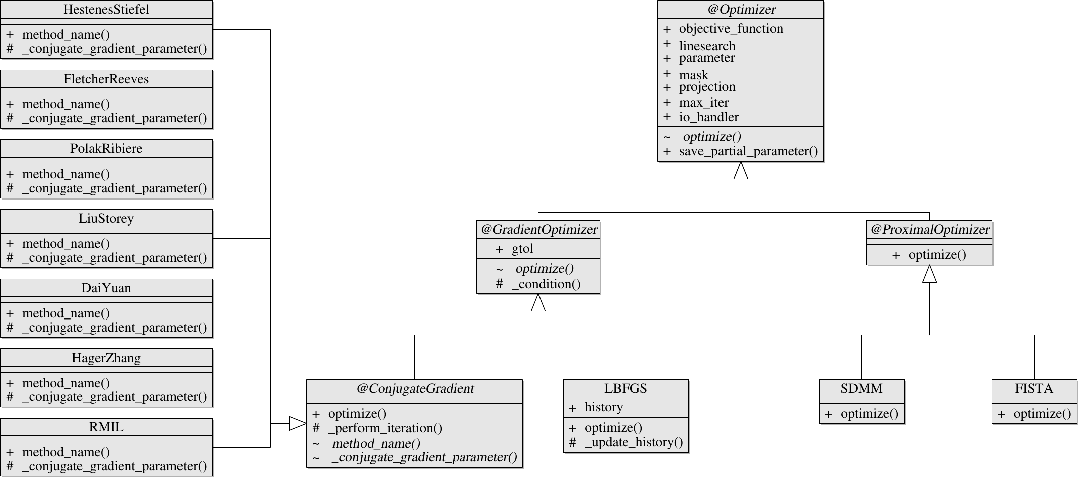
**Optimizer hierarchy** (`Optimizer`, gradient/proximal optimizers, and CG/LBFGS families).#

Note

Proximal optimizers FISTA and SDMM are covered in Compressed Sensing & Proximal Methods. They use FISTABacktracking and optional Step Size Seeders rather than the Armijo line searchers attached to CG/L-BFGS.

Overview#

Gradient-based optimizers#
Optimizer	Type	Description	Robustness	Speed	Memory	Typical use case
Hestenes-Stiefel	CG	Strong global convergence, nonlinear problems	Medium	Fair	Low	Nonlinear, large-scale
Fletcher-Reeves	CG	Classic CG, quadratic problems	Medium	Fair	Low	Nonlinear, large-scale
Polak-Ribiere	CG	Dynamic gradient update	Medium	Good	Low	Nonlinear, large-scale
Liu-Storey	CG	Image restoration, unconstrained problems	Medium	Good	Low	Image restoration
Dai-Yuan	CG	Performance-oriented CG scaling	Medium	Fair	Low	Nonlinear, large-scale
Hager-Zhang	CG	Modern nonlinear CG, stable and fast	High	Good	Low	Preferred CG choice
RMIL	CG	Sufficient descent, image recovery	Medium	Good	Low	Denoising, image recovery
LBFGS	Quasi-Newton	Limited-memory BFGS	High	Best	Medium	Default for smooth imaging

Practical selection

Start with LBFGS for most smooth imaging problems.
Prefer HagerZhang when memory for L-BFGS history is tight but a quasi-Newton step is not required.
Other CG variants are available for experimentation or when their theoretical properties match the problem.

References: [Dai and Yuan, 1999, Fletcher and Reeves, 1964, Hager and Zhang, 2005, Hestenes and Stiefel, 1952, Liu and Storey, 1991, Nocedal and Wright, 2006, Polak and Ribière, 1969, Polyak, 1969, Rivaie et al., 2012]

Common setup#

Every gradient optimizer needs:

A reconstructed parameter (usually an Image).
An ObjectiveFunction (see Objective Function Framework and Optimization in Pyralysis).
A Line Searchers instance (optionally with a Step Size Seeders).

from pyralysis.optimization.linesearch import BacktrackingArmijo, BarzilaiBorweinAlternating
from pyralysis.optimization.optimizer import LBFGS

seeder = BarzilaiBorweinAlternating(min_step=1e-10)
ls = BacktrackingArmijo(objective_function=of, seeder=seeder)

optim = LBFGS(
    parameter=image,
    objective_function=of,
    linesearch=ls,
    max_iter=100,
    io_handler=ioh,
)
reconstructed = optim.optimize()

Conjugate gradient methods#

All CG classes inherit from ConjugateGradient. At iteration \(k\) the search direction is

\[d_k = -g_k + \beta_k \, d_{k-1}\]

where \(g_k = \nabla f(x_k)\). The line searcher finds \(\alpha_k\) along \(d_k\); see Line Searchers.

Gradient / line-search convention

ObjectiveFunction.dphi follows: search_direction = -dphi. After calculate_gradient(), dphi holds \(g\). CG sets dphi = -d before the line search so the 1D objective f1dim sees a consistent sign.

Restart strategy#

When either condition holds, \(\beta_k = 0\) (steepest descent step) [Powell, 1977]:

Negative beta: \(\beta_k \leq 0\).
Powell restart: \(g_{k+1}^T g_k < \eta \|g_{k+1}\|^2\) with \(\eta = 0.2\).

CG variants and \(\beta_k\) formulas#

HestenesStiefel#

\[\beta_k^{\mathrm{HS}} = \frac{g_{k+1}^T (g_{k+1} - g_k)}{(g_{k+1} - g_k)^T d_k}\]

FletcherReeves#

\[\beta_k^{\mathrm{FR}} = \frac{\|g_{k+1}\|^2}{\|g_k\|^2}\]

PolakRibiere#

\[\beta_k^{\mathrm{PRP}} = \frac{g_{k+1}^T (g_{k+1} - g_k)}{\|g_k\|^2}\]

LiuStorey#

\[\beta_k^{\mathrm{LS}} = -\frac{(g_{k+1} - g_k)^T g_{k+1}}{g_k^T d_k}\]

DaiYuan#

\[\beta_k^{\mathrm{DY}} = \frac{\|g_{k+1}\|^2}{(g_{k+1} - g_k)^T d_k}\]

HagerZhang#

With \(y_k = g_{k+1} - g_k\):

\[\beta_k^{\mathrm{HZ}} = \frac{y_k^T g_{k+1}}{d_k^T y_k} - 2 \frac{\|y_k\|^2 (d_k^T g_{k+1})}{(d_k^T y_k)^2}\]

RMIL#

\[\beta_k^{\mathrm{RMIL}} = \frac{g_{k+1}^T (g_{k+1} - g_k)}{d_k^T (d_k - g_k)}\]

Per-optimizer examples#

from pyralysis.optimization.optimizer import HagerZhang, FletcherReeves, RMIL

optim = HagerZhang(
    image=image,
    objective_function=of,
    linesearch=ls,
    max_iter=100,
    io_handler=ioh,
)
result = optim.optimize()

LBFGS (limited-memory BFGS)#

Class: LBFGS

Quasi-Newton method that approximates the inverse Hessian using the most recent max_corrections pairs \((s_i, y_i)\) without forming the full matrix.

Key parameters

Parameter	Default	Role
`max_corrections`	`10`	Max \((s,y)\) pairs (RAM + disk combined)
`memory_threshold_gb`	`100.0`	Switch vectorized vs sequential two-loop
`use_disk_storage`	`False`	Spill pairs to Zarr when `in_memory_limit` is set
`in_memory_limit`	`None`	Max pairs kept in RAM when spilling enabled

max_corrections=0 reduces to steepest descent with the same line search and stopping rules.
Pairs are accepted only if \(\Re(y^H s) > 0\); \(\rho = 1/\Re(y^H s)\) uses a dtype-aware machine epsilon floor.

Memory optimizations

Lazy deque allocation for correction pairs.
Hybrid vectorized/sequential two-loop recursion based on memory_threshold_gb.
Optional Zarr-backed spill for very large images.
Cached \(\gamma\) scaling and consistent Dask chunking across history.

from pyralysis.optimization.optimizer import LBFGS

optim = LBFGS(
    parameter=image,
    objective_function=of,
    linesearch=ls,
    max_iter=100,
    io_handler=ioh,
    max_corrections=10,
)

# Large images: spill older pairs to disk
optim = LBFGS(
    parameter=large_image,
    objective_function=of,
    linesearch=ls,
    max_iter=100,
    max_corrections=10,
    use_disk_storage=True,
    in_memory_limit=5,
    memory_threshold_gb=50.0,
)

Saving intermediate results#

Pass an I/O handler to write intermediate images during optimize() with partial_parameter=True. The optimizer passes the live Image to the handler; host/device conversion is the handler’s job (see Partial parameter snapshots (optimization) in I/O Operations & Data Formats).

from pyralysis.io import FITS
from pyralysis.io.zarr import ZarrArray

# FITS or ZarrArray — both accept CuPy-backed Dask Images from GPU runs
ioh = FITS(use_dask=True)   # or ZarrArray()
optim = LBFGS(
    parameter=image,
    objective_function=of,
    linesearch=ls,
    io_handler=ioh,
)
optim.optimize(
    partial_parameter=True,
    partial_parameter_interval=10,  # partial_10, partial_20, ...; final always saved
)

Implementation notes#

All CG variants support complex parameters with stable inner products.
GradientNormError is raised when the gradient norm vanishes (convergence or degeneracy).
CG conjugate_gradient_parameter returns host scalars to avoid redundant .compute() calls.

Dask iterate state (custom optimizers)#

Gradient optimizers assign a new lazy parameter.data each iteration (line search, acceleration, or quasi-Newton update). Dask then accumulates graph lineage on the carried iterate unless it is collapsed before the next loop. Without that step, memory and scheduler overhead grow linearly with iteration count and can OOM on large images.

Built-in optimizers call _finalize_iteration_state() at the end of each iteration. It persists Dask-backed parameters in place (no-op for NumPy) via persist().

When implementing a new optimizer, call _finalize_iteration_state on every Parameter you carry to the next iteration (primary iterate; FISTA also finalizes the accelerated point y_k). For carried state stored as raw dask.array.Array objects, use _finalize_dask_arrays() instead (SDMM does this for z and u each outer iteration). This is independent of optional caches such as ObjectiveFunction.persist_gradient (aggregate gradient) or LBFGS direction / correction-pair persistence (multi-reuse within one iteration).

from pyralysis.optimization.optimizer import Optimizer

class MyOptimizer(Optimizer):
    def optimize(self):
        x = self.parameter
        for k in range(self.max_iter):
            # ... compute search direction, line search, assign x.data ...
            x = updated_param
            self._finalize_iteration_state(x)
        return x

See Performance & Scalability for the full persist policy (gradient, proximal, LBFGS history, SDMM auxiliary variables).

Progress vs diagnostics#

Optimizer iteration lines (Iteration N, function value, step size, convergence) are progress output, not diagnostic logs:

Use verbose=True/False on optimize() to gate them.
Internally they go through pyralysis.runtime.logging.progress, which uses dask.distributed.print when a Distributed client is active (so lines appear once on the client) and built-in print otherwise.
Do not expect to silence iteration lines with logging levels alone.

Diagnostics (I/O warnings, setup failures, debug traces) use pyralysis.runtime.logging.get_logger / the standard logging module. Configure the pyralysis logger from a CLI or notebook entry point with configure_logging(level="DEBUG") when you need subsystem detail without treating progress as INFO.

[1]

Yu-Hong Dai and Yaxiang Yuan. A nonlinear conjugate gradient method with a strong global convergence property. SIAM Journal on Optimization, 10(1):177–182, 1999. doi:10.1137/S1052623497318992.

[2]

Roger Fletcher and Colin M. Reeves. Function minimization by conjugate gradients. The Computer Journal, 7(2):149–154, 1964. doi:10.1093/comjnl/7.2.149.

[3]

William W. Hager and Hongchao Zhang. A new conjugate gradient method with guaranteed descent and an efficient line search. SIAM Journal on Optimization, 16(1):170–192, 2005. doi:10.1137/030601880.

[4]

Magnus R. Hestenes and Eduard Stiefel. Methods of conjugate gradients for solving linear systems. Journal of Research of the National Bureau of Standards, 49(6):409–436, 1952. doi:10.6028/jres.049.044.

[5]

Y. Liu and C. Storey. Efficient generalized conjugate gradient algorithms, part 1: theory. Journal of Optimization Theory and Applications, 69(1):129–137, 1991. doi:10.1007/BF00940464.

[6]

Jorge Nocedal and Stephen J. Wright. Numerical Optimization. Springer, 2 edition, 2006. doi:10.1007/978-0-387-40065-5.

[7]

E. Polak and G. Ribière. Note sur la convergence de méthodes de directions conjuguées. Revue Française d'Informatique et de Recherche Opérationnelle, 3(R1):35–43, 1969.

[8]

Boris T. Polyak. The conjugate gradient method in extreme problems. USSR Computational Mathematics and Mathematical Physics, 9(4):94–112, 1969. doi:10.1016/0041-5553(69)90035-4.

[9]

M. J. D. Powell. Restart procedures for the conjugate gradient method. Mathematical Programming, 12(1):241–254, 1977. doi:10.1007/BF01593790.

[10]

Mohd Rivaie, Mustafa Mamat, Lidya Ismail, and Ali Abashar. A new class of nonlinear conjugate gradient coefficients with global convergence properties. Applied Mathematics and Computation, 218(22):11323–11332, 2012. doi:10.1016/j.amc.2012.05.030.